Quantifying Epistemic Uncertainty with the Laplace Approximation

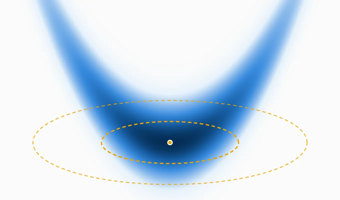
Modern neural networks are remarkably good at giving answers — and remarkably bad at telling you when those answers shouldn’t be trusted. A trained network hands you a single point estimate of its weights, and with it a single prediction, delivered with the same unwavering confidence whether the input looks like the training data or like nothing the model has ever seen. This is a problem of epistemic uncertainty: uncertainty that stems not from noise in the data, but from our own ignorance about which model is actually correct given the finite data we’ve observed.

The Bayesian approach to this problem is conceptually clean. Rather than committing to one set of weights, maintain a posterior distribution over all of them, and let predictions reflect the spread of that posterior. The difficulty is that the exact posterior over millions of parameters is intractable, and common approximations such as deep ensembles, variational inference, and MCMC require either multiple training runs or a different training pipeline.

The Laplace approximation avoids both requirements. The idea is to take a network that has already been trained, treat its weights as the mode of the posterior, and fit a Gaussian around that mode whose covariance is determined by the local curvature of the loss. In one post-hoc step, a deterministic network becomes an approximate Bayesian one.

What is the Laplace approximation?

The intuition is easiest to see with a single weight. Imagine a curve that scores every possible value of that weight by how well it explains the training data. Training climbs this curve and finds the highest point: the single best value, which we call $\theta_\text{MAP}$.

But the shape of the curve around the peak tells us something the point alone cannot. If the peak is sharp and narrow, only values very close to $\theta_\text{MAP}$ explain the data well, so we can trust that value. If the peak is broad and flat, many different values would have worked nearly as well, and picking just one hides real uncertainty about which is correct.

The Laplace approximation captures this shape with a single measurement: how quickly the curve drops off as we move away from the peak. From that measurement, it builds a bell curve centered on $\theta_\text{MAP}$ — a narrow bell for a sharp peak, meaning high confidence, and a wide bell for a flat peak, meaning low confidence. That bell curve is a Gaussian distribution over the weight, and its width is the epistemic uncertainty we were missing.

In technical terms: the curve that scores each weight value is the log posterior, how sharply it falls away from the peak is its curvature, and fitting the bell curve is a quadratic approximation at the mode.

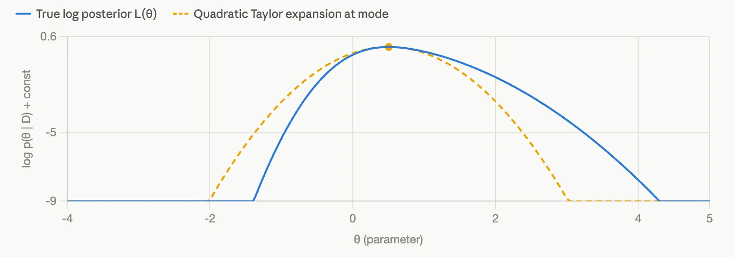
Figure 1: The Laplace approximation fits a quadratic to the true log posterior at the mode. The two match in value, slope, and curvature at $\theta_\text{MAP}$, and diverge as we move away. That divergence is the approximation error.

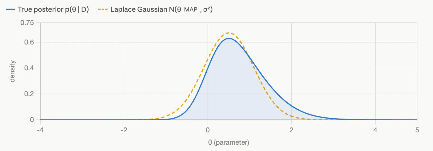
Figure 2: Converting the log posterior back into a distribution turns the quadratic into a Gaussian. The Laplace approximation is exact when the true posterior is Gaussian, and remains a faithful local description around the mode even when the true posterior is skewed and the Gaussian misplaces some mass in the tail.

The rest of this post makes this picture precise, and extends it from one weight to all of them.

Hessian of the loss

Consider a classification problem with training data $D = \{(x_i,y_i)\}_{i=1}^N$ and model parameters $\theta$. With $f_\theta(x)$ denoting the output logits, the predicted class is the one with the highest softmax score. The softmax spread over classes is commonly read as aleatoric uncertainty, the uncertainty inherent to the data. The trained model itself, however, is deterministic: it provides no signal about how uncertain we should be about the model, so the epistemic uncertainty is missing entirely. See our Capsa page for an explanation of the different types of uncertainty.

The Laplace approximation recovers this missing signal. The starting point is to recognize that the training loss is, up to a constant, the negative log posterior over the weights: the data-fit term is the negative log likelihood, and the weight-decay regularizer corresponds to a Gaussian prior,

$$\mathcal{L}(D;\theta) = -\log p(D|\theta) - \log p(\theta).$$

We take a second-order Taylor expansion of the loss around the trained weights $\theta_\text{MAP}$:

$$\mathcal{L}(D; \theta) \approx \mathcal{L}(D; \theta_\text{MAP}) + \frac{1}{2}(\theta - \theta_\text{MAP})^\top H(\theta - \theta_\text{MAP}),\,\,\,\,\,H=\nabla_\theta^2 \mathcal{L}(D;\theta)\big|_{\theta_\text{MAP}}.$$

The first-order term vanishes because the gradient is zero at the MAP estimate — this is precisely why the expansion must be centered at a trained optimum. What remains is a quadratic bowl whose curvature is the Hessian $H$.

The posterior is proportional to the exponentiated negative loss, $p(\theta|D) \propto e^{-\mathcal{L}(D;\theta)}$. Exponentiating the negative of our quadratic gives exactly the functional form of an (unnormalized) Gaussian density, so we can write:

$$p(\theta|D) \approx \mathcal{N}(\theta; \theta_\text{MAP}, \Sigma),\,\,\,\,\,\,\Sigma = H^{-1}.$$

The covariance $\Sigma$, the inverse curvature, represents our uncertainty about the weights. The geometry is intuitive: flat directions in the loss landscape, where many weight configurations explain the data equally well, have small curvature and therefore large posterior variance; sharply curved directions pin the weights down and yield confident beliefs.

From weight uncertainty to output uncertainty

A Gaussian over millions of weights is not, by itself, the signal we want — we care about uncertainty in the model’s outputs. The standard route is the linearized Laplace approximation: linearize the network around $\theta_\text{MAP}$,

$$f_\theta(x) \approx f_{\theta_\text{MAP}} (x) + J(x) (\theta - \theta_\text{MAP}),$$

where $J(x)=\nabla_\theta f_\theta(x)\big|_{\theta_\text{MAP}} \in \mathbb{R}^{C\times P}$ is the Jacobian of the $C$ logits with respect to the $P$ parameters. The Jacobian is the bridge between weight space and output space: pushing the Gaussian posterior through this linear map gives a Gaussian over the logits, with covariance

$$\text{Cov}(f_\theta(x)) = J(x) \Sigma \,J(x)^\top.$$

This is the epistemic uncertainty signal. Inputs that resemble the training data produce Jacobians aligned with well-constrained (high-curvature) directions of the posterior, yielding small logit variance. Inputs far from the training distribution excite poorly constrained directions, and the variance grows — the model is telling us it doesn’t know.

Somewhat surprisingly, linearizing is not just a computational convenience: predictions from the linearized model are often better calibrated than sampling weights from the Laplace posterior and pushing them through the full nonlinear network (Improving Predictions of Bayesian Neural Nets via Local Linearization, Immer et al., AISTATS 2021), because the linearization is consistent with the local Gaussian assumption that produced $\Sigma$ in the first place.

Converting this logit-space uncertainty into predictive probabilities is straightforward, either by sampling logits from the Gaussian and averaging their softmax outputs, or via a simple closed-form correction. In both cases, where the logit variance is large, the predictive distribution is pulled toward uniform, so the model’s confidence decreases as inputs move away from the training distribution.

In summary: the Laplace approximation reads the model’s uncertainty about its own weights from the shape of the loss surface at the trained optimum, and the linearization step translates that weight uncertainty into a per-input uncertainty on the model’s outputs. Inputs the training data constrained well receive low epistemic uncertainty; inputs that depend on poorly constrained weights receive high uncertainty.

Does it work?

We took a BERT classifier fine-tuned on the SNLI natural language inference dataset and fit a Laplace approximation to the trained model, with no retraining and no change to the model itself. We then evaluated it under distribution shift using MNLI, a multi-genre inference dataset that poses the same task as SNLI but draws its text from different domains.

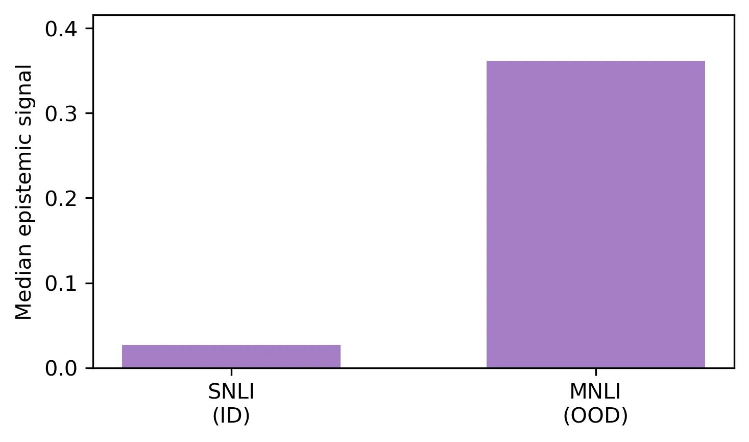
Figure 3: Median per-input epistemic signal on in-distribution (SNLI) and out-of-distribution (MNLI) data. For each input, we sample logits from the Gaussian predictive given by the linearized Laplace approximation and measure how much the resulting confidence in the predicted class varies across samples; the bars show the median of this signal over each dataset.

If the sampled logits all lead to the same confident prediction, the epistemic uncertainty at that input is negligible and the signal is near zero; if they disagree, the prediction is sensitive to directions the training data never constrained, and the signal is large. This is the pattern we observe: on in-distribution data the signal is close to zero, since these inputs resemble what the model was trained on, while on out-of-distribution data the median signal is more than an order of magnitude larger. The model assigns high epistemic uncertainty to unfamiliar inputs before any label is available to indicate an error.

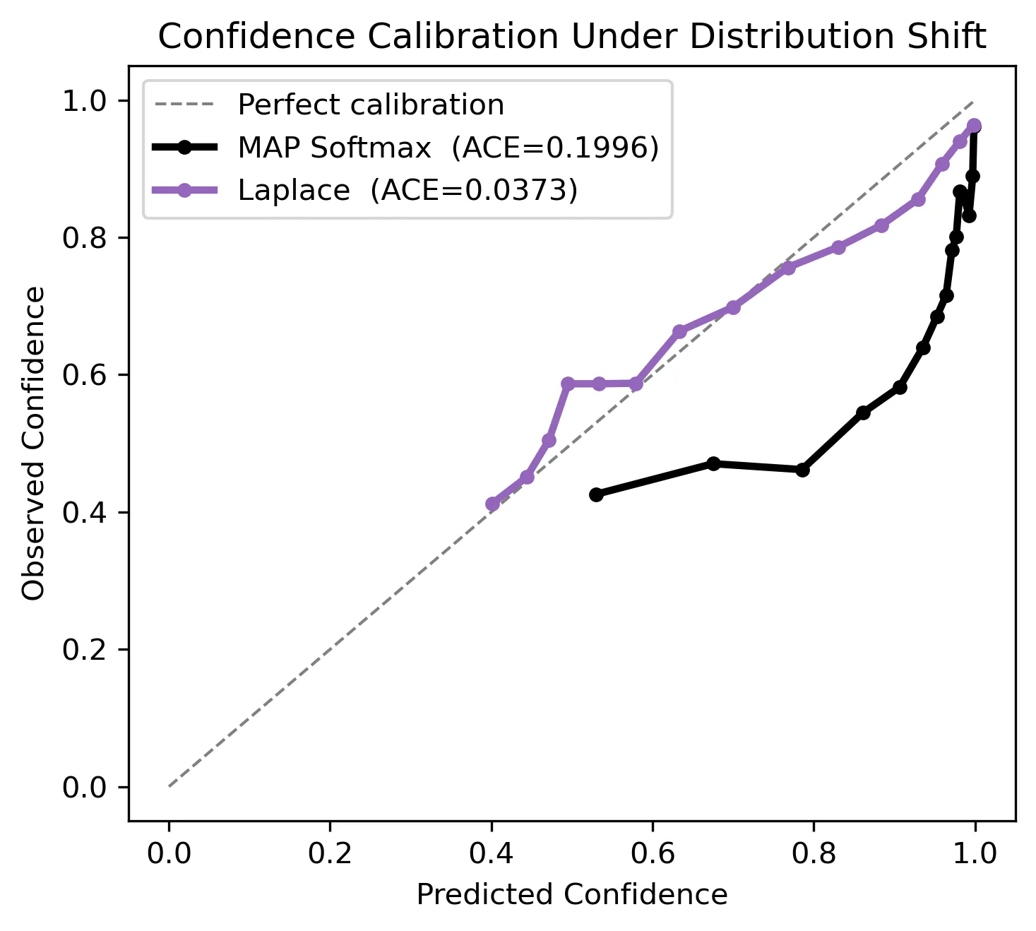
Figure 4: Reliability diagram on out-of-distribution data (MNLI). Predictions are grouped into bins by their stated confidence (x-axis); for each bin we plot the fraction that were actually correct (y-axis). A perfectly calibrated model lies on the diagonal: when it says “80% confident,” it is right 80% of the time.

Under distribution shift, the deterministic model’s softmax confidence is severely miscalibrated. The black curve sits far below the diagonal: the model claims high confidence on inputs it frequently gets wrong, and predictions made with roughly 80% confidence are correct less than half the time. The Laplace-corrected predictions track the diagonal closely, reducing the adaptive calibration error (ACE, the equal-mass-bin variant of the standard expected calibration error) from 0.200 to 0.0373, achieved entirely post hoc. The model’s stated confidence becomes a quantity that downstream decisions can rely on.

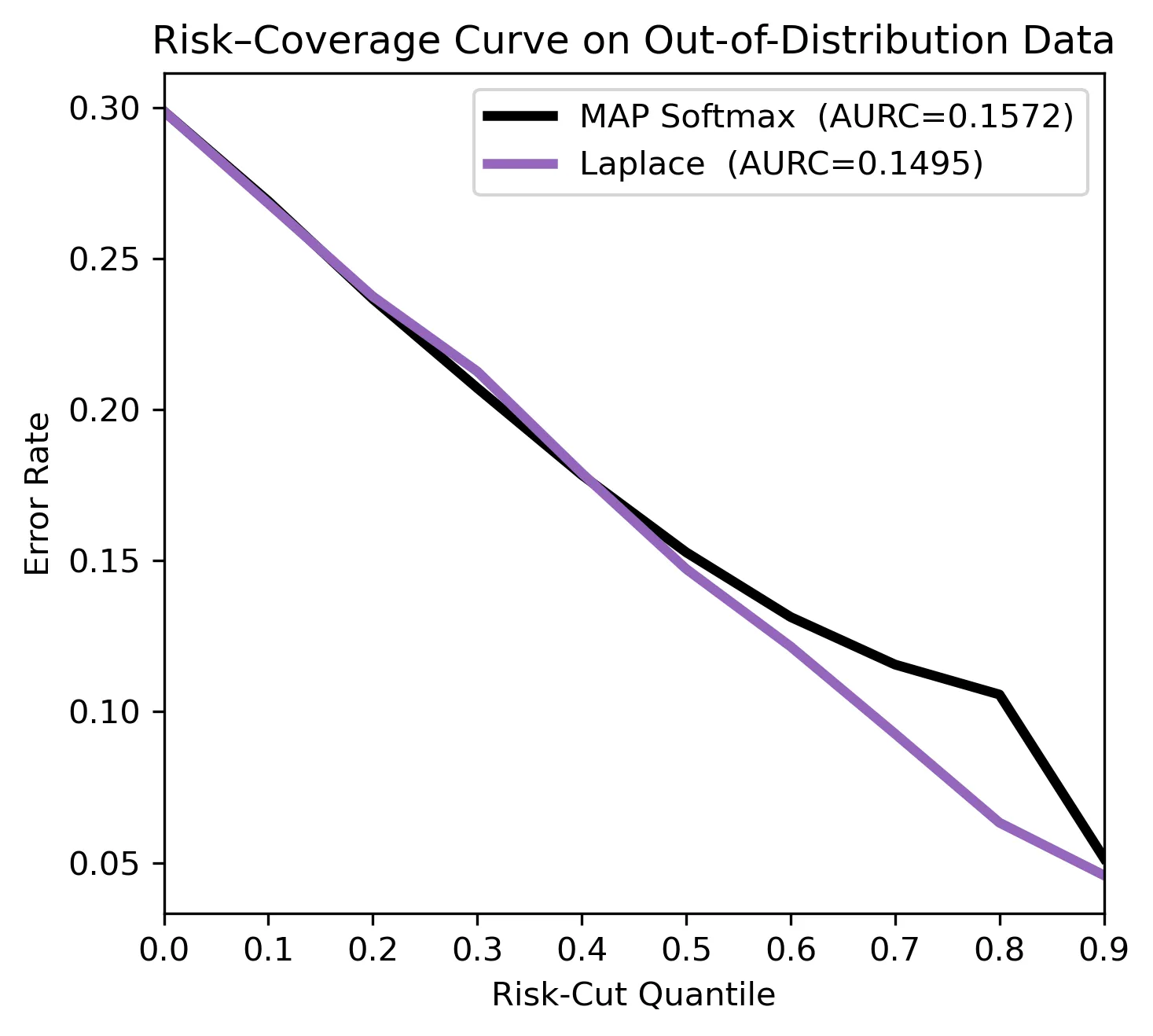
Figure 5: Risk-coverage curve on out-of-distribution data (MNLI). Each curve shows how the error rate falls as the model abstains on its least-confident inputs: the x-axis is the fraction of inputs removed (ranked from most to least uncertain), the y-axis is the error rate on the predictions that remain. Each method ranks inputs by its own uncertainty signal, so a curve that drops faster indicates a signal that is better at identifying which predictions are wrong.

Removing uncertain inputs reduces error under both signals, but the Laplace uncertainty ranks errors more effectively, achieving a lower area under the risk-coverage curve (AURC 0.150 vs. 0.157). The curves briefly cross in the mid-quantiles, likely due to ranking noise on borderline examples, but the overall trend favors Laplace, and the advantage widens at higher abstention rates: beyond 50% abstention the Laplace curve stays consistently below the baseline, and at 80% abstention the error rate on retained predictions is roughly half that of the softmax baseline.

The takeaways: a trained network’s loss landscape already contains an epistemic uncertainty signal, and the Laplace approximation extracts it without retraining. In our experiments this signal identifies unfamiliar inputs (Figure 3), corrects the model’s overconfidence under distribution shift (Figure 4), and supports an abstention policy that trades coverage for reliability (Figure 5).

A trade worth making

The Laplace approximation has three properties that matter for deployment:

1. It is post hoc: no retraining and no change to the training pipeline, since it attaches to an existing trained model.
2. It is cheap: a single pass over the trained model, with none of the overhead of ensembles.
3. It is sufficient: as the results above show, the tasks production systems require (flagging unfamiliar inputs, calibrating confidence, deciding when to abstain) do not demand a perfect posterior. The local geometry at the trained optimum carries sufficient signal for all three.

These properties come at the cost of some theoretical fidelity, concentrated in one simplifying assumption: the posterior is described by a single Gaussian at a single mode. It does not capture multimodality (if two distant weight configurations both explain the data, Laplace represents only one of them), and it can misplace probability mass when the local loss landscape is heavily skewed or non-quadratic.

The gap between the equations above and a working system is also real. The Hessian of a modern network is far too large to form, let alone invert; computing per-input Jacobians efficiently requires care; and the quality of the resulting uncertainties depends on implementation choices (which curvature approximation to use, which parts of the network to treat as uncertain, how to set the prior) that the math leaves open.

These choices are well studied in the literature, but getting them right for a given model and deployment is engineering work. Turning uncertainty methods into production-ready tools is exactly what we build Capsa for: wrappers that attach uncertainty estimation to an existing model without touching its training pipeline.